00:00:00
let's start basic lecture one
00:00:03
in this lecture you will learn about the
00:00:05
geometry and radiation source definition
00:00:12
the goal of this training is to
00:00:14
understand the basic format of the fits
00:00:16
input file set the basic system and
00:00:18
radiation source and be able to execute
00:00:21
particle transport simulation
00:00:24
this is the simulation result at the end
00:00:26
of this training
00:00:27
it shows the particle fluence in the
00:00:29
system when a 290 mev proton beam is
00:00:32
incident on a cylindrical water
00:00:39
the contents of the training are shown
00:00:41
here
00:00:42
the order of the contents of this
00:00:44
training will be general description
00:00:46
geometry source summary and homework
00:00:54
here is the format of the fits input
00:00:56
file
00:00:57
all calculation conditions are described
00:01:00
by text input
00:01:01
the input file consists of multiple
00:01:04
sections and the section name and square
00:01:06
brackets indicates the beginning of the
00:01:08
section
00:01:09
the basic format of the input file is
00:01:11
represented by a keyword or parameter
00:01:14
equal to a numerical value or a
00:01:16
character string
00:01:18
at this time the space is ignored
00:01:21
alternatively it is represented by a
00:01:23
list of numbers or character strings
00:01:26
at this time please note that it is
00:01:28
separated by spaces up to 200 characters
00:01:32
can be put on one line and more than
00:01:34
that it should be on the continuation
00:01:36
line and the continuation line should
00:01:38
have six or more spaces at the beginning
00:01:41
of the sentence
00:01:42
it is also possible to give parameters
00:01:45
as mathematical formulas
00:01:50
here is the input assistance
00:01:53
by turning off the section name you can
00:01:55
skip the section
00:01:57
when you write qp colon at the line head
00:02:00
reading of parameters is skipped from
00:02:02
this line to the next section
00:02:04
q colon is equivalent to the n section
00:02:07
any input information written below the
00:02:10
n section is ignored
00:02:12
to add a comment in an input file please
00:02:14
add c in the first five columns of a
00:02:17
line except the material section and
00:02:19
dollar and hash in the middle of a line
00:02:22
but please avoid using hash in the cell
00:02:25
and surface sections
00:02:27
considering the above we recommend using
00:02:30
the dollar mark for comment marks
00:02:38
here is shown the main components of
00:02:40
input file
00:02:42
in the fit simulation geometry in
00:02:44
three-dimensional virtual space and
00:02:46
information on source particles are both
00:02:49
essential to tally various quantities of
00:02:51
the particles
00:02:53
they are three fundamental components
00:02:55
please open and see input example of
00:02:58
lex01 inp
00:03:06
this slide shows the configuration of
00:03:08
the sample input of lex01.inp
00:03:12
this input file consists of nine
00:03:14
sections
00:03:15
the material surface and cell sections
00:03:17
define the three-dimensional virtual
00:03:19
space
00:03:20
the source section defines the
00:03:22
production of particles
00:03:24
the track tally and 3d show tally define
00:03:27
the observation of quantities
00:03:33
here the file obtained by the
00:03:35
calculation of this example is shown
00:03:38
batch dot out shows the progress of the
00:03:41
calculation
00:03:42
details will be explained in basic
00:03:44
lecture three fits dot out shows a
00:03:47
summary file of fits calculation results
00:03:51
i will briefly introduce it later
00:03:53
the remaining files are image and
00:03:55
numerical data files of calculation
00:03:58
results and statistical errors
00:04:01
details will be explained in basic
00:04:03
lecture two
00:04:04
here is an example of terminal output
00:04:07
it includes input file name and
00:04:09
calculation progress and time
00:04:11
information
00:04:13
if there is an error in the input file
00:04:15
error information may be output
00:04:22
this is an eps file that shows the image
00:04:24
display of the calculation result and a
00:04:27
summary file that shows the summary of
00:04:29
the calculation
00:04:36
here is the standard output file
00:04:39
the first part of the fits out file is
00:04:41
fits logo and version information
00:04:44
the second part is the input echo
00:04:47
in this part parameters specified in the
00:04:49
input file are shown with description of
00:04:52
the parameters and their default values
00:04:55
the third part is the memory status in
00:04:57
which you can check how many memories
00:04:59
are used in the calculation
00:05:02
the fourth part is the batch information
00:05:05
and the last part is the summary of fit
00:05:07
simulation
00:05:08
in the last part you can check these
00:05:11
information that is numbers of events
00:05:13
such as source generation and nuclear
00:05:16
reaction information on transported
00:05:18
particles numbers of secondary particles
00:05:22
cpu time and numbers of library data
00:05:25
access and use of reaction models
00:05:28
it should be noted that error
00:05:29
information is mostly given in the
00:05:31
console window but occasionally in the
00:05:34
output file
00:05:37
this indicates the section type
00:05:40
various sections are provided to
00:05:42
faithfully reproduce the actual
00:05:43
experimental conditions
00:05:46
please see section 5 of the manual for
00:05:48
each section
00:05:49
[Music]
00:05:51
here is shown the list of tally
00:05:54
several tallies can be defined in one
00:05:56
calculation to obtain various
00:05:58
information on the particle transport
00:06:01
the detail for each tally section is
00:06:03
described in the fits manual
00:06:05
and it will also be introduced in the
00:06:07
basic lecture number two
00:06:11
next is general definition of geometry
00:06:18
here is shown general definition of
00:06:19
geometry
00:06:21
to make a three-dimensional geometry
00:06:23
following three steps are required
00:06:26
first you define materials in material
00:06:29
section
00:06:30
second you define surfaces of cells in
00:06:33
surface section
00:06:34
and then you define cells by combining
00:06:37
of material and surface in cell section
00:06:47
in the fits calculation cells are
00:06:49
defined in xyz coordinate system
00:06:52
you can use an infinite space
00:06:55
however void and air regions have to be
00:06:57
defined explicitly
00:06:59
furthermore the outer boundary of the
00:07:01
virtual space so called outer void has
00:07:04
to be defined
00:07:06
the outer void work as a cutoff region
00:07:09
that is when particle enter the outer
00:07:11
void transport calculation of the
00:07:13
particle is finished
00:07:19
here is shown how to define materials
00:07:22
the format of definition is material
00:07:24
number symbol for element and
00:07:27
composition ratio
00:07:29
for example this line defines two
00:07:31
hydrogen and one oxygen that is water
00:07:34
for material number one
00:07:36
you can define composition ratio as
00:07:39
atomic ratio and mass ratio by changing
00:07:42
sign of ratio positive composition ratio
00:07:45
means atomic ratio and negative
00:07:48
composition ratio means mass ratio
00:07:51
it should be mentioned that when
00:07:52
elements are specified without mass
00:07:54
number natural isotopic composition is
00:07:57
assumed
00:07:59
following formats are available to
00:08:01
specify the mass number
00:08:03
you can use element symbol with mass
00:08:05
number and formula with atomic number
00:08:07
and mass number
00:08:12
now let's see how to define a surface
00:08:15
the format of definition is surface
00:08:17
number shape and parameters
00:08:20
for example this line defines surface of
00:08:23
sphere having its center at the origin
00:08:25
of the xyz coordinate system with a
00:08:27
radius of 10 centimeter
00:08:29
note that parameters are in units of
00:08:31
centimeter
00:08:32
there are various types of surface
00:08:34
shapes that is sphere plane cylinder
00:08:38
rectangular and so on
00:08:44
next slide shows how to define cells
00:08:47
the format of definition is cell number
00:08:50
material number density and surface
00:08:52
numbers for example this line defines
00:08:56
the cell with the number of 100 which
00:08:58
filled by water with the density of 1.0
00:09:01
gram per cubic centimeter and the region
00:09:04
is inside surface 10.
00:09:06
when material density is over 1 the unit
00:09:09
of atom density is 10 to the 24 atoms
00:09:12
per cubic centimeter
00:09:14
when material density is less than 1 the
00:09:17
unit of atom density is gram per cubic
00:09:19
centimeter
00:09:21
the next line defines cell number the
00:09:23
outer void cell and outside surface tin
00:09:27
when you define void density is not
00:09:29
necessary
00:09:34
now let's confirm the geometry defined
00:09:37
in the input file
00:09:39
please open the lex01 inp file by your
00:09:42
text editor
00:09:44
the procedure to confirm your geometry
00:09:46
is as follows
00:09:48
at first change ic and tl parameter in
00:09:51
the parameters section
00:09:53
please set eight for eye control when
00:09:56
you confirm the geometry
00:09:58
next overwrite save the input file and
00:10:01
execute fits
00:10:03
after that open an eps file track xcx
00:10:06
and you can see like this figure
00:10:13
let's start exercise one
00:10:16
in this step please change the radius of
00:10:18
the sphere to 20 centimeter
00:10:21
the left side shows a part of input file
00:10:23
and the red underline points the
00:10:25
parameter that have to be changed
00:10:28
after editing the input file please
00:10:30
execute fits and check the output file
00:10:33
please start the exercise
00:10:41
here is the answer
00:10:43
the cell 100 is defined by surface 10
00:10:46
so we change the radius of the surface
00:10:48
from 10 centimeters to 20 centimeters
00:10:52
after that you will obtain this result
00:11:01
this slide shows example of error
00:11:03
message from input file
00:11:06
if you fail to run fits the line number
00:11:08
where the mistake was made and its
00:11:10
contents are displayed in the terminal
00:11:12
window
00:11:13
it may be output to fits out
00:11:16
in this case please check the contents
00:11:19
of the corresponding line number and
00:11:21
correct the input file
00:11:26
here is shown about the input file
00:11:29
every lecture of fits tutorial has a lot
00:11:31
of exercises but only one or a few input
00:11:35
files are included in each folder
00:11:38
if you would like to skip some exercises
00:11:40
you can use the input files in input
00:11:42
folder such as select 1-2 inp
00:11:46
for example if you would like to try the
00:11:49
exercise 3 please use select 1-3 inp in
00:11:53
the input folder
00:11:55
this input file includes all the
00:11:57
revisions that have been done in the
00:11:59
exercises 1 and 2.
00:12:04
in this slide let's define a new surface
00:12:07
please define a spherical surface whose
00:12:10
radius is 5 centimeter and center is at
00:12:13
the origin of the xyz coordinate system
00:12:16
the surface number of the new surface is
00:12:18
11.
00:12:19
in this step we just define the surface
00:12:22
thus geometry does not change
00:12:31
in the exercise 2 please add a new
00:12:34
spherical water cell with 5 centimeter
00:12:36
radius to the system
00:12:38
let's use 102 for new cell number
00:12:41
let's start with this exercise
00:12:50
if you defined the cell 102 like that
00:12:53
you obtained the result as shown here
00:12:56
this is because part of cell 100
00:12:58
overlaps cell 102
00:13:01
the overlapped regions is painted in
00:13:03
black
00:13:04
this is one of typical errors in cell
00:13:06
definition
00:13:08
fits always identifies the region in
00:13:10
which the particle is crossing so fits
00:13:12
get confused when one location is doubly
00:13:15
defined
00:13:22
when a geometry error occurs fits
00:13:24
outputs an error file to provide
00:13:26
detailed information on the error
00:13:29
the contents of error file is shown here
00:13:32
there are cell numbers
00:13:34
error is observed there
00:13:37
these are x y z coordinates where the
00:13:39
geometry error occurs
00:13:42
information at multiple coordinate
00:13:44
points is exported even if only one
00:13:46
error has occurred
00:13:52
the other type of geometry error is
00:13:55
undefined region
00:13:56
geometry is defined in an infinite space
00:13:59
but every single point must be filled
00:14:01
with certain materials or defined as a
00:14:04
void
00:14:05
undefined regions is painted in purple
00:14:08
if undefined region is present the other
00:14:11
region does not appear sometimes
00:14:16
next proceed to the method of defining
00:14:19
cells
00:14:23
the topic of this subject is how to
00:14:24
define cells
00:14:26
cells are defined by surface using plus
00:14:29
and minus signs and boolean operators
00:14:32
at first plus sign on the surface number
00:14:35
means the outside of the surface and
00:14:37
minus sine means the inside of the
00:14:39
surface
00:14:40
boolean operators are used when you
00:14:42
define cell by combined use of more than
00:14:45
two surfaces
00:14:46
the detail will be shown in the next
00:14:48
slides
00:14:54
here is shown the boolean operator and
00:14:58
to define a sail inside or outside of
00:15:00
two surfaces connect the two number with
00:15:03
a blank it means and
00:15:06
so in the case of exercise 2 the cell
00:15:09
100 are defined by inside of surface 10
00:15:12
and outside of surface 11
00:15:15
and then we will obtain the answer as
00:15:17
shown here
00:15:18
so please try and check it
00:15:27
next here is shown the boolean operator
00:15:30
not
00:15:31
when you want to excluded cells from the
00:15:33
other cell you can use hash mark it
00:15:36
means not
00:15:37
you can define cell 100 by using not
00:15:40
like that
00:15:41
it means the cell 102 is excluded from
00:15:44
the inside of the surface tin thus they
00:15:46
are equivalent
00:15:48
it should be noted that cells are
00:15:50
usually defined by using surface number
00:15:52
but hash mark must be followed by a cell
00:15:55
number
00:15:56
when you use surface numbers with hash
00:15:58
mark you have to set surface numbers
00:16:00
inside round bracket
00:16:02
this will be explained later
00:16:06
before we go on the next exercise we
00:16:08
will extend the virtual space
00:16:11
three-dimensional virtual space should
00:16:13
be large enough to contain all the
00:16:15
geometrical components
00:16:17
so let's change the radius of surface
00:16:20
102 to 500 centimeters
00:16:23
after that you will get the result like
00:16:26
this figure
00:16:31
now let's start exercise three
00:16:34
in this exercise we will add sphere cell
00:16:37
103 having its center in the xyz
00:16:40
coordinate 0 0 11 with radius of 5
00:16:43
centimeters
00:16:45
here the symbol for surface shape is s z
00:16:48
when you define the sphere on the z axis
00:16:51
so please execute and check where is
00:16:53
cell 103
00:16:55
let's start it
00:17:01
the cell 103 will placed on the right
00:17:04
side of cell 102.
00:17:06
here spheres are defined with symbols of
00:17:09
sx psi and sz when center of sphere is
00:17:13
placed on the axis
00:17:15
the universal expression s is used with
00:17:18
the x y z coordinate of its center and
00:17:20
its radius
00:17:24
in the next exercise we will change the
00:17:27
center of cell 103 inches to z equals
00:17:29
eight inches
00:17:31
when the cell is moved two spheres are
00:17:33
overlapped and geometry error will occur
00:17:37
so please exclude this overlap regions
00:17:39
from cells 102 and 103 and create a new
00:17:43
cell 104
00:17:48
here is shown an example of the answers
00:17:52
cell 104 is added and it defined inside
00:17:55
of surface 11 and surface 12.
00:17:58
these surfaces are excluded from both
00:18:00
cell 102 and cell 103
00:18:04
cell 104 is also excluded from cell 100
00:18:08
newly added cells have to be excluded
00:18:10
from the background cell
00:18:16
here is shown the boolean operator o r
00:18:19
to define a sum of two regions as a cell
00:18:22
connect the two numbers with signs by
00:18:24
colon it means o r
00:18:27
it is an example for excluding cell by
00:18:29
using colon
00:18:31
these expressions give same result
00:18:34
it should be mentioned that you have to
00:18:35
use surface numbers inside round break
00:18:38
kit after hash mark
00:18:45
here is shown a bad example using
00:18:47
unnecessary hash marks
00:18:49
this is an onion geometry which are
00:18:51
constructed by five sphere surface like
00:18:54
onion
00:18:55
if you define this geometry by using
00:18:57
hash mark input file becomes long
00:19:01
while input file can express simpler by
00:19:03
using and and or operators
00:19:12
next is definitions of boxes and
00:19:14
cylinders
00:19:17
this slide shows how to make a box
00:19:20
boxes can be defined using rpp which is
00:19:23
rectangular parallelopiped
00:19:26
this surface needs six parameters to set
00:19:28
minimum and maximum of xyz coordinates
00:19:32
please note that rpp is defined in the
00:19:35
surface section because rpp corresponds
00:19:38
to 6 surfaces of the box
00:19:44
let's start with exercise 5.
00:19:47
now let's define a 10 centimeter cube
00:19:49
centered at 0 0 minus 11 using symbol of
00:19:53
rpp
00:19:55
first set a cube in the range of minus 5
00:19:58
centimeters to 5 centimeters for x and y
00:20:01
directions and minus 16 centimeters to
00:20:04
minus 6 centimeters for z direction
00:20:07
then in the cell section define the
00:20:09
inside of the surface specified by rpp
00:20:12
as a cell using a minus symbol
00:20:15
let's execute fits and see the result to
00:20:17
confirm whether a cube is correctly
00:20:19
defined or not
00:20:23
here is the answer
00:20:24
at first rpp surface is defined in
00:20:28
surface section
00:20:30
and then cell 105 is defined as an
00:20:33
inside of surface 13 and this cell is
00:20:36
excluded from cell 100
00:20:44
this slide shows you how to divide cells
00:20:46
by a plane in the surface section we can
00:20:49
also define plane
00:20:51
the symbol of px means perpendicular
00:20:54
plane to x-axis
00:20:56
the numerical parameter of px means
00:20:58
where the plane is placed on
00:21:00
in the cell section we use symbols plus
00:21:03
or minus to distinguish the two regions
00:21:06
divided by a plane
00:21:08
so now let's add red texts and then
00:21:11
execute
00:21:14
fits this is the result
00:21:17
the cell 102 is defined as an inside of
00:21:20
the surface 11 and outside of the
00:21:23
surface 12 and negative region of the
00:21:25
surface 14.
00:21:27
that is the positive region of the
00:21:29
surface 14 in the sphere with the five
00:21:32
centimeter radius is cut
00:21:34
p y and pz are also available
00:21:37
be careful of the meaning of plus and
00:21:40
minus when you use planes
00:21:44
here is shown how to make a cylinder
00:21:47
a cylinder is defined using an infinite
00:21:49
cylindrical tube and two planes
00:21:56
now let's define a cylinder in exercise
00:21:59
6.
00:22:00
please add red texts in the surface and
00:22:02
cell sections
00:22:04
in the surface section symbol of cz
00:22:06
means parallel cylindrical tube to
00:22:09
z-axis
00:22:10
the numerical parameter of cz is the
00:22:13
radius of tube
00:22:14
in the cell section please define a
00:22:16
cylinder as a cell 106.
00:22:19
the inside and outside correspond to
00:22:22
minus and plus symbols
00:22:25
since the cell 106 overlaps the cells
00:22:28
100 102 103 104 and 105 new cells should
00:22:35
be excluded from these cells
00:22:37
let's execute fits and see the result to
00:22:39
confirm whether a cylinder is correctly
00:22:42
defined or not
00:22:46
here is the answer
00:22:48
cell 106 is a cylinder with a radius of
00:22:52
1 centimeter and a height of 38
00:22:54
centimeters
00:22:56
and the cylinder 106 pierces all regions
00:23:09
for cell and surface definition we
00:23:11
recommend to rearrange cell and surface
00:23:13
numbers according to own rules
00:23:16
for example rearrange the numbers in
00:23:18
ascending order in each plane surfaces
00:23:28
next is shown how to add materials
00:23:33
in this subject we learn how to add
00:23:35
materials
00:23:37
you can add a new material number and
00:23:39
define a composition ratio of the
00:23:41
material in material section
00:23:44
please note that the density is give in
00:23:46
the cell section
00:23:48
when you write symbol of element without
00:23:50
atomic number its natural isotope ratio
00:23:53
is used
00:23:55
we can also define mixtures and
00:23:57
compounds as shown here
00:24:02
now let's start the exercise 7.
00:24:05
please add copper in the material
00:24:07
section and change the material in the
00:24:10
cell 106 from water to copper
00:24:13
the density of copper is 8.93 gram per
00:24:16
cubic centimeter at first define the
00:24:19
material number two
00:24:21
and then change the definition of cell
00:24:23
106
00:24:25
note that each material number has own
00:24:27
color
00:24:28
after that please execute fits and check
00:24:31
the result
00:24:34
here is the answer
00:24:36
at first copper is added in the material
00:24:39
section
00:24:40
when you write symbol of element without
00:24:42
atomic number its natural isotope ratio
00:24:45
is used
00:24:47
next the material number and density for
00:24:49
cell 106 is changed
00:24:52
and then you get this result
00:24:58
let me go on the next slide
00:25:00
here is shown how to make a void cell
00:25:03
the material number for void is zero and
00:25:06
material number for outer void is minus
00:25:08
one
00:25:09
when you set void cells the densities
00:25:12
should be skipped so please define the
00:25:15
cell 100 as void and then execute fits
00:25:18
the right figure is the result
00:25:21
you can see that color of cell 100
00:25:23
changed
00:25:28
with the material name color section you
00:25:31
can change the colors of cells and
00:25:33
specify the name and color of each
00:25:35
material number
00:25:36
let's add material name color section
00:25:39
and let one inp and execute fits
00:25:42
after that you can obtain this figure
00:25:48
this slide shows the color definition
00:25:50
you can use these colors in the material
00:25:53
name color section
00:25:58
next is shown geometry drawing software
00:26:04
this slide shows about confirmation of
00:26:06
geometry with fig 3d
00:26:08
here fig 3d is fits interactive geometry
00:26:11
viewer in 3d which is an input geometry
00:26:14
visualization software for fits
00:26:17
let's see the geometry by using fig 3d
00:26:21
for windows we can right click the fits
00:26:24
input file and select send to and fig 3d
00:26:28
for mac os we can drag and drop the fits
00:26:31
input file to the fig 3d icon in the
00:26:34
dock
00:26:35
for linux we can move to the folder with
00:26:38
the fits input file and type big 3d fits
00:26:41
inp in the terminal
00:26:46
here is how to cut of a cross section
00:26:48
with an auxiliary plane
00:26:50
click the settings tab to display the
00:26:52
auxiliary plane display
00:26:55
x y and z are planes perpendicular to
00:26:58
the x-axis y-axis and z-axis
00:27:02
respectively
00:27:03
select enable or disable for cutting
00:27:05
plane in the check box
00:27:07
you can also select cut of the plus side
00:27:10
minus side with the radio button
00:27:13
finally press the draw button to display
00:27:15
the cross section in this figure
00:27:21
here is how to select cells for
00:27:23
visualization
00:27:25
when you click the cell pane the list of
00:27:27
cells is displayed
00:27:29
when you uncheck cell 102 and click the
00:27:31
draw button the material of cell 102 is
00:27:34
disappeared
00:27:42
here is shown how to change the colors
00:27:44
first please select tools configuration
00:27:47
color in the menu bar
00:27:49
then you can select colors of background
00:27:52
or materials in the color tab
00:27:55
after that click the ok
00:27:57
these setting parameters correspond to
00:28:00
the matte name color section section
00:28:02
changing the colors is also available
00:28:05
with a matte name color section
00:28:10
here is shown super mc
00:28:12
it is a free software developed by the
00:28:14
fds team at the chinese academic of
00:28:17
science
00:28:18
registration is required when you get it
00:28:21
it convert cad geometry into several
00:28:24
monte carlo code format
00:28:26
compatible cad formats are set sab stp
00:28:30
and step
00:28:32
the sample of super mc and pits are
00:28:34
placed in this directory but instruction
00:28:36
only available in japanese at the moment
00:28:42
from here let's learn how to define
00:28:44
radiation source
00:28:49
to define the radiation source we have
00:28:51
to set the source section
00:28:53
this is the second main component of the
00:28:56
fits input file
00:29:00
here types of sources are shown
00:29:03
it says several source types
00:29:06
so we have to select the type in
00:29:08
accordance with each purpose
00:29:10
for example point isotropic source is
00:29:13
suitable for simulating radioisotope
00:29:16
facilities
00:29:17
for accelerator facilities pencil or
00:29:20
broad beam along specified direction or
00:29:23
cone beam source is suitable
00:29:25
for radioactive waste and internal
00:29:27
exposure volume isotropic source should
00:29:30
be set
00:29:31
for cosmic ray and external exposure
00:29:34
isotropic irradiation within certain
00:29:37
area is used
00:29:41
in this slide four points to define the
00:29:43
source section are shown
00:29:45
the first one is shape of source
00:29:47
distribution
00:29:49
this means spatial distributions
00:29:52
point cylinder sphere etc are available
00:29:56
next is energy of source particles
00:29:59
mono energies or continuum spectra can
00:30:01
be set
00:30:03
the third one is source particle species
00:30:06
we can set neutron photon proton heavy
00:30:09
ion etc
00:30:11
the last is direction of source
00:30:13
particles
00:30:14
isotropic directional cone shape etc can
00:30:18
be set
00:30:22
let's see the source section of
00:30:23
lex01.inp
00:30:26
the source section is used to define the
00:30:28
source particle of the simulation
00:30:31
the first parameter is s type
00:30:34
when setting s type equals 1 a
00:30:36
cylindrical shape is set as a region for
00:30:39
generating source particles
00:30:41
what information is required to define a
00:30:43
cylinder
00:30:45
parameters in the blue line box are used
00:30:47
to define a cylinder shape
00:30:52
this slide shows several parameters to
00:30:54
define a cylinder source
00:30:56
first the default direction of fits is
00:30:59
plus z
00:31:00
so a central axis of the cylinder is z
00:31:03
axis
00:31:05
r0 is a radius of the cylinder
00:31:08
z0 and z1 are respectively minimum and
00:31:12
maximum of z coordinates
00:31:14
the height of the cylinder is determined
00:31:16
by these parameters
00:31:18
x0 and y0 are respectively x and y
00:31:22
coordinates of the central axis
00:31:24
these parameters are optional and their
00:31:27
default values are zero
00:31:29
r1 is also optional when you set this
00:31:32
parameter the inner region is removed
00:31:35
and then the source region like pipes
00:31:37
can be set
00:31:41
when setting s type equals 1 we can
00:31:44
define not only cylinder shape source
00:31:46
but also circle and point shape sources
00:31:49
in this slide red arrows mean directions
00:31:52
of source particles
00:31:54
when we set isotropic source the
00:31:56
directions are randomly determined like
00:31:58
this the center and right figures are
00:32:01
examples of extension of the cylinder
00:32:03
shape
00:32:04
when you set z zero equals z one for
00:32:07
example z zero equals five and z one
00:32:10
equals five the shape of the source
00:32:13
becomes a disk
00:32:14
furthermore by setting r0 equals zero
00:32:18
the shape of the source becomes a point
00:32:20
note that source disks or points should
00:32:22
not be set on boundaries of cells
00:32:25
because numerical errors sometimes occur
00:32:27
when running a fit simulation
00:32:31
let's try exercise eight
00:32:33
execute a transport calculation of bits
00:32:37
please change i control parameter to
00:32:39
zero in the parameters section check r0
00:32:43
z0 and z1 parameters in the source
00:32:46
section
00:32:47
these settings mean point source at the
00:32:49
origin 0 0 0
00:32:53
furthermore please check the t-track
00:32:55
section 2.
00:32:57
although we will learn the detail of
00:32:58
this section in the second basic lecture
00:33:01
here please set nt equals 10 and then
00:33:04
execute fits
00:33:06
this t-type setting gives output of
00:33:08
transport simulation of 10 pages
00:33:11
after running this please open the track
00:33:13
xzx file
00:33:15
each page means an output of the
00:33:17
transport simulation from 0 to 1
00:33:20
nanosecond in 0.1 nanoseconds increments
00:33:30
this is answer of the excise 8.
00:33:32
this red line in track xzx means
00:33:35
trajectory of source proton particles
00:33:38
these protons were generated at the
00:33:40
origin and then moved along the z-axis
00:33:44
their direction is plus z and the length
00:33:46
of this trajectory is short because
00:33:48
proton is a charged particle
00:33:54
next let's make a disk source with a
00:33:56
radius of one centimeter
00:33:58
in this case please change our zero
00:34:01
parameter
00:34:08
this is answer nine
00:34:10
by setting r zero equals one the width
00:34:13
of the red beam was spread out
00:34:16
because the radius is one centimeter the
00:34:18
width is two centimeters
00:34:24
next point is energy setting of source
00:34:27
particles
00:34:28
mono energy can be defined by e0
00:34:31
it should be mentioned that the unit of
00:34:33
energy is mev per nucleons
00:34:36
please remember this unit is important
00:34:38
for heavy ions
00:34:40
of course this is mev for protons or
00:34:43
neutrons
00:34:44
when we set energy spectrum the
00:34:46
distribution is defined by e type
00:34:49
subsection
00:34:50
this subsection is not explained here
00:34:52
but we can learn it in source a of the
00:34:54
advanced lecture
00:34:59
the third point is source particle
00:35:01
species
00:35:02
by pro projectile parameter we can
00:35:05
define the particle species
00:35:07
we can use symbol or kf code to define
00:35:10
it
00:35:11
this table shows the symbol and kf code
00:35:14
for each particle the symbol format is
00:35:17
usually used in the definition
00:35:20
nucleus is specified by mass number and
00:35:22
element symbol for example 12c for
00:35:25
carbon 12 ions
00:35:27
it should be mentioned that when we use
00:35:29
radioisotope sources we have to specify
00:35:32
the emitted particle species such as
00:35:35
photon
00:35:36
kf code is special expression in
00:35:38
elementary physics
00:35:40
this is not used usually but we have to
00:35:43
use this format for example when
00:35:46
simulating neutrino transport
00:35:51
next is exercise 10
00:35:54
let's change the source particle to
00:35:56
neutrons with energies of 100 mev
00:35:59
we can solve this problem by changing
00:36:02
pro and e0 parameters
00:36:10
this is answer
00:36:11
by setting pri equals neutron and e0
00:36:14
equals 100 we can obtain the result of
00:36:17
the neutron source simulation like this
00:36:20
these neutrons can penetrate the
00:36:22
material unlike protons
00:36:28
the last point is direction of source
00:36:30
particles
00:36:32
the direction is defined in the
00:36:33
spherical coordinate system and z-axis
00:36:36
is the default direction in fits
00:36:39
the parameter dir means polar angle phi
00:36:42
means as a muffle angle and dom means
00:36:45
beam spread
00:36:46
the main parameter is d i r
00:36:49
this is cosine of the angle between the
00:36:51
pointing direction and the z axis
00:36:54
therefore d i r equals 1 means the angle
00:36:58
theta equals 0 degree or d i or equals 0
00:37:01
means that theta equals 90 degrees
00:37:04
as a special setting d i r equals all
00:37:07
means isotropic source
00:37:13
next slide shows how to set phi
00:37:15
parameter
00:37:16
phi is as a muffle angle and is given in
00:37:19
units of degrees
00:37:21
please be careful this unit because that
00:37:23
of d ir is different
00:37:25
phi is given as counterclockwise angle
00:37:27
between the plus x axis and the
00:37:29
projection onto the x y plane
00:37:32
for example when we set the direction
00:37:35
tilted by 45 degrees from the plus x
00:37:38
axis on the x y plane we have to set d
00:37:41
ir equals zero and phi equals 45.
00:37:47
the last one is dom parameter
00:37:50
dom means solid angle
00:37:53
the unit is degree
00:37:55
when we define a beam spread of 30
00:37:57
degrees we should set dom equals 30.
00:38:04
here is shown the relation of parameters
00:38:06
dir phi and dom in the spherical
00:38:09
coordinate system
00:38:13
let's move on the next exercise
00:38:16
please define an isotropic point source
00:38:19
at the x y z coordinate 0 0 10
00:38:23
please change four parameters above red
00:38:26
lines
00:38:27
when s type equals 1 we can define an
00:38:30
isotropic source by setting d ir equals
00:38:33
all
00:38:40
this is answer of the exercise
00:38:43
the answers are d ir equals all r0
00:38:46
equals 0 and both c0 and z1 equal 10.
00:38:51
please see the right panel
00:38:53
we can find that the red point is at the
00:38:55
coordinate 0 0 10 and the direction of
00:38:59
the neutron source is isotropic
00:39:05
so let me summarize the basic lecture
00:39:08
number one
00:39:13
this is summary of the basic lecture one
00:39:16
the main components of a fifth input
00:39:18
file are geometry source and tally
00:39:22
geometry is defined by the three
00:39:24
sections material surface and cell
00:39:27
sections and we can define various 3d
00:39:30
geometrical components based on the gg
00:39:33
general geometry concept
00:39:36
source is defined by four points shape
00:39:39
species energy and direction of
00:39:41
particles
00:39:43
tally is used to calculate the
00:39:45
quantities in fits radiation transport
00:39:47
calculation
00:39:49
this will be explained in the basic
00:39:51
lecture 2.
00:39:57
let's try this homework
00:39:59
please use an input file homework one
00:40:02
inp in a folder shown in this slide
00:40:05
in this homework we have to make a water
00:40:08
cylinder and then irradiate it by a
00:40:10
proton beam at 290 mev
00:40:14
there are several hints in these slides
00:40:16
please try this problem step by step
00:40:35
you