00:00:00
hello i'm mrs wilkins and welcome to
00:00:02
marsbury science
00:00:03
today we're going to look at an a-level
00:00:05
physics-required practical how to
00:00:07
determine the young modulus of a
00:00:08
material and specifically a copper wire
00:00:11
the young modulus is a really important
00:00:13
property in engineering as it tells us
00:00:15
how easily a material will stretch or
00:00:17
deform the young modulus is defined as
00:00:19
the ratio of tensile stress to tensile
00:00:22
strain where stress is the force applied
00:00:25
per unit area and the strain is the
00:00:27
extension relative to original length
00:00:30
the young modulus is given the letter e
00:00:32
and this is equal to f l
00:00:35
over a delta l this is the setup that
00:00:38
we're going to use today we have taken a
00:00:41
fairly long piece of copper wire it is
00:00:43
over two meters because the extensions
00:00:45
are so small you do want fairly long
00:00:47
original length this is just one example
00:00:50
of a setup you can also hang some wires
00:00:53
sometimes steel is the best vertically
00:00:56
suspended from a beam but it depends if
00:00:57
your school laboratory has that sort of
00:00:59
infrastructure that enables you to do it
00:01:01
so this is the best option for us in
00:01:03
this investigation there are two safety
00:01:05
precautions to consider the first is
00:01:08
that if the wire breaks and it may well
00:01:11
do it could snap across the surface of
00:01:14
the eye causing damage so it is really
00:01:17
important to wear eye protection in the
00:01:19
form of safety goggles this second is
00:01:22
that if the wire snaps of course the
00:01:24
slot masses will force the ground
00:01:26
be careful not to have your foot or a
00:01:28
knee underneath the slot masses and
00:01:31
perhaps also place a carpet or a tray of
00:01:33
sand underneath the slot masses to
00:01:35
protect the floor when they fall so the
00:01:38
fourth applied is the tension that we
00:01:40
apply to the wire as you can see we have
00:01:42
clamped the wire at the far end of the
00:01:44
bench and then we've run the wire over a
00:01:46
pulley and attached it to a vernier
00:01:49
scale at the end of the vernier scale we
00:01:50
have the hanger and we are going to
00:01:54
attach slot masses in increments of 100
00:01:56
grams and that will provide the tension
00:01:59
which is mg you will notice that we
00:02:01
actually have two wires attached and
00:02:03
this is because it's important to have a
00:02:05
test wire that we apply the tension
00:02:08
force to and also a comparison wire this
00:02:11
allows us to give us a reference point
00:02:13
and also if there are any changes in the
00:02:15
ambient atmosphere for example if the
00:02:17
wire extends due to temperature it will
00:02:19
happen to both and we can find the
00:02:21
relative extension of the test wire the
00:02:23
next step is to find the diameter of the
00:02:25
wire and for this the best equipment is
00:02:27
a micrometer and this will give us a
00:02:29
resolution to a hundredth of a
00:02:30
millimeter the wire may not be perfectly
00:02:33
uniform throughout and so it's a good
00:02:35
idea to take the diameter measure the
00:02:36
diameter at three separate points and
00:02:39
then calculate the mean i'm going to
00:02:41
take it here
00:02:42
you
00:02:43
turn the small dial until you hear the
00:02:45
first click
00:02:47
and i can see the reading
00:02:48
to be
00:02:51
0.28 millimeters i then measured the
00:02:54
diameter in the middle of the wire and
00:02:56
at the far end of the wire
00:02:58
the first two readings were the same the
00:03:00
diameter was 0.28 millimeters but the
00:03:02
third was 0.27 millimeters however when
00:03:05
i calculated the mean you still have to
00:03:07
give the final result to two significant
00:03:10
figures and so it still averages out
00:03:12
2.28 millimeters cross sectional area
00:03:14
equals pi d squared over four the next
00:03:17
measurement we require is the original
00:03:19
length of the wire and for this we used
00:03:22
a series of meter rules and found the
00:03:24
original length to be 2.46 meters we
00:03:27
have of course already applied a small
00:03:29
tension to the wire to ensure that the
00:03:31
wire is taught when we took the readings
00:03:33
of diameter and original length and this
00:03:35
was supplied by the hangers already
00:03:37
attached to the vernier scale
00:03:39
however before we add the additional 100
00:03:42
grams we have to make sure that our
00:03:44
vernier scale is perfectly zeroed so if
00:03:47
we go back to our original equation e
00:03:49
equals f l over a delta l we've
00:03:52
accounted for the force we've measured
00:03:53
the original length we've calculated the
00:03:55
cross-sectional area by measuring the
00:03:57
diameter so now we can start to measure
00:03:59
the extension under an applied force by
00:04:02
attaching the slot masses and we will
00:04:06
measure the extension on the vernier
00:04:07
scale so i'm going to start by adding my
00:04:10
first 100 grams because this is our
00:04:12
reference point of zero as i mentioned
00:04:14
before the extensions are very small and
00:04:17
so far i have not seen a significant
00:04:19
extension so i'm going to add another
00:04:21
100 grams i've taken a few readings now
00:04:24
and i can see that adding 500 grams is
00:04:28
now ascended by 1.4 millimeters if
00:04:32
you're not sure how to read vernier
00:04:33
scales remember that there are two
00:04:34
scales the first reading you see where
00:04:37
the zero on the sliding scale where it's
00:04:40
between on the fixed scale so i can see
00:04:42
it's between one and two millimeters so
00:04:44
i know it's one point something
00:04:46
millimeters i then get the next decimal
00:04:49
point by seeing which is the first line
00:04:52
that lines up with a line on the fixed
00:04:54
scale and i can see here that the fourth
00:04:57
line lines up with the fixed scale and
00:05:00
therefore i can say it's 1.4 millimeters
00:05:02
in this investigation although we're
00:05:04
interested in extension in meters our
00:05:06
vernier scale gives us an extension in
00:05:08
millimeters so don't forget to convert
00:05:10
it to meters when plotting your graph
00:05:12
when you have a full set of data we can
00:05:15
now plot the graph there are various
00:05:17
ways of plotting the graph and you could
00:05:18
plot the stress versus the strain but
00:05:20
this is quite a complicated way of doing
00:05:22
it it's more standard to plot the force
00:05:25
against extension however plotting a
00:05:27
force when you have to times the mass by
00:05:29
g 9.81 the values aren't particularly
00:05:32
easy to plot on a graph so we're going
00:05:34
to stick with the mass and the extension
00:05:37
our preferred method is to plot the mass
00:05:39
on the y-axis and the extension on the
00:05:42
x-axis because this gives us quite a
00:05:44
typical stress-strain curve that you'd
00:05:47
be familiar with if you plot the
00:05:50
extension on the y-axis and the mass on
00:05:52
the x-axis which you may also see it
00:05:54
does of course give you the inverse for
00:05:56
the gradient plotting it this way our
00:05:59
gradient gives us the mass divided by
00:06:01
delta l we can then say that the young
00:06:04
modulus e is equal to the gradient
00:06:07
times g times the original length
00:06:10
divided by the cross-sectional area
00:06:12
when measuring the gradient it's really
00:06:14
important that you take the gradient
00:06:16
from the linear part of the graph
00:06:19
your graph may show a linear part and
00:06:21
then it may curve off in which case
00:06:23
that's great because you've shown that
00:06:25
the wire behaves elastically and then
00:06:28
starts to behave plastically
00:06:30
however for determining young modulus
00:06:32
it's really important to only take the
00:06:34
gradient in the linear part and not
00:06:37
include the part after it's gone beyond
00:06:39
the limit of proportionality it's also
00:06:41
important on your graph to plot the mass
00:06:43
in kilograms our gradient is 357
00:06:46
kilograms per meter times that by g 9.81
00:06:51
times it by our original length which
00:06:52
was 2.46 meters and divided by our
00:06:55
cross-sectional area which was 6.2 times
00:06:58
10 to the minus 8 meter squared and we
00:07:00
get a value for the young's modulus e of
00:07:03
1.39 x 10 to the 11 pascals
00:07:07
or 139 giga pascals we can compare this
00:07:11
to the known value of the young modulus
00:07:13
of copper which is
00:07:15
gigapascals we can now take a percentage
00:07:18
error in our value compared to the
00:07:20
theoretical value which gives us a
00:07:22
percentage error of 19 percent